One of the most important research breakthroughs in the 20th century was the laser. Lasers are ubiquitous and used everywhere from navigation to bar code scanners to high-precision experiments. But before examining the specifics of state-of-the-art laser technology, let us first go over the essential quantum theory behind how lasers work.
A review of stimulated and spontaneous emission
We encountered and briefly discussed the phenomenon of stimulated emission that underlies lasers, but let us review the topic again to gain greater familiarity for the heavy quantum theory that follows.
Remember that stimulated emission is one of two modes of light emission (the emission of photons, the quantum particle associated with light). The other, more “conventional” way that atoms emit photons is the process of spontaneous emission. This is a three-step process[1]:
An atom absorbs a photon, and is excited to a higher-energy state with energy
The atom then decays to a lower-energy state, which has energy .
A new photon is released in the process, with energy and wavelength
Spontaneous emission is how most light (which includes UV, infrared, microwave, radio wave, etc.) in the universe is produced, from starlight to incandescent lightbulbs[2]. It has several important characteristics:
The decay from the upper state to the lower state happens spontaneously, without anything to trigger it.[3]
Although the decay rate (probability of a decay) can be predicted, when exactly the decay occurs is random.
The photons that are emitted from the decay travel in random directions and their polarization, frequency, and wavelength cannot be predicted in advance
Spontaneous emission is not helpful for building a laser, because there is no way to pre-determine the characteristics of the photon to be emitted. Thus, spontaneously-emitted light is not monochromatic (monochromatic means that the light is of only one frequency), but rather, spread across a wide range of frequencies, and the emitted photons travel away in random directions[4], meaning that the light is not collimated and cannot form a tight beam. These two undesirable results defeat the point of a laser, where we want to produce light of a single frequency in a tightly-focused beam.
But there exists an alternative means of light emission, known as stimulated emission. Stimulated emission is also a multi-step process, but with different steps:
An atom is excited by some external energy source (this can be in the form of electric, electromagnetic/light, chemical, thermal or even nuclear energy). The energy source raises the atom into a higher-energy state with energy .
The already-excited atom absorbs a photon that also has energy
The atom then decays down to a lower-energy state, which has energy .
Two identical photons are released in the process, each with energy and thus wavelength
Crucially, stimulated emission is different from spontaneous emission in the following ways:
The atom is already in an upper state even before a photon strikes the atom, due to the external energy source
This means that two photons are emitted from the decay, unlike in spontaneous emission, where only a single photon is released
The two emitted photons are identical, with the same predictable frequency and direction
We call this process stimulated emission due to the fact that this entire process is stimulated due to the energy source. Since the atom emits two photons, the two outgoing photons can then strike two new atoms, which each emit two photons, which is four photons total. This doubling process continues, as four photons becomes eight photons becomes sixteen photons, causing a continuous chain reaction. Even better, the resulting light produced is monochromatic and in the same direction, which are fantastic for building lasers!
Operating principles of lasers
After our conceptual review, let us reformulate what we know about light emission and absorption in a more rigorous, mathematical way. Again, we know from the quantum model of the hydrogen atom that electrons can have different states. As each state is an eigenstate of the Hamiltonian, different states (usually) have different energies. If an atom absorbs a photon, for instance, the atom can jump from its lower-energy state, which we write as , to a higher-energy upper state, which we write as . Meanwhile, an atom can also decay to its lower state by emitting a photon, with the difference in the energies between the upper state and the lower state being the energy of this photon. While atoms, in general, have a multitude of states (and more than one upper state), this two-state approximation is good enough for a lot of theoretical analysis. A diagram of the two-state atomic system is shown below:
An atomic system with two possible states ( and ). A transition from to is accompanied by the emission of a photon with energy .
Whether the photon is emitted via stimulated emission or spontaneous emission, precisely when the decay happens is random. We do know, however, that this process follows a probabilistic law, first derived by Einstein in 1916. Let us assume we are studying a certain group of atoms. Let be the expected number of atoms in a higher energy state . Over time, these electrons will spontaneously decay to a lower energy state , such that follows the differential equation:
Where is called the Einstein A coefficient, and is approximately the probability that an atom will decay from per unit time. Remember, this is probabilistic, as in is the expected number of electrons in the upper state, as in, it is most likely that at time there are electrons that are in the upper state . This differential equation is just an exponential decay whose solution is:
Remember that spontaneous emission is fundamentally random in nature; they follow general probabilistic rules but those are simply probabilities. But we don’t want that, we want emission of photons that we can control.
For this, we need stimulated emission. First, we bring the atom to its upper state by surrounding it with an externally-applied energy source. When this energy source is another electromagnetic field (e.g. flash lamp, arc lamp, sunlight, even an LED) is called optical pumping. It is in fact possible to use one laser to optically pump another laser - in fact, this is often the most efficient method of pumping a laser, and can be used to take a laser beam of one wavelength to be able to produce a laser beam of another wavelength.
The wavelength used in optical pumping does not necessarily have to be the same wavelength that is emitted. The chief requirement is that the optical source used in optical pumping matches one of the absorption lines of the atom (or molecule, or molecular gas lasers). For instance, hydrogen absorbs (and correspondingly, also emits) wavelengths of 656 nm (red), 486 nm (cyan), 434 nm (blue), 410 nm (violet), and a variety of other wavelengths in the UV band, among others, as shown below:
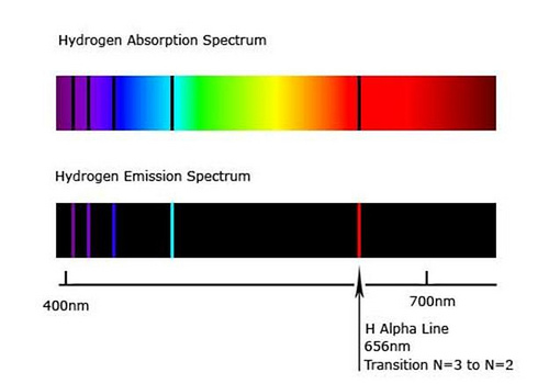
The spectrum of hydrogen, showing the wavelengths of light hydrogen absorbs and emits. Black lines, also called spectral lines, indicate atomic transitions.
But while these absorption lines at the most well-known, they are not its only absorption lines, because, due to fine structure and hyperfine structure (the splitting of energy levels due to complex quantum effects), other types of transitions are possible, including the 21 cm absorption line (and emission line) in the microwave spectrum.
When an atom has been raised to its upper state by some energy source, a passing photon that has energy will stimulate the decay of the atom from its excited-state to its ground-state , releasing another further photon of energy with the exact same properties as the passing photon. The passing photon that stimulated the transition between the states, however, is not absorbed, meaning that now there are two photons of energy . These two photons can then pass by one atom each, triggering the release of two more photons from each atom, so four photoms after. The process continues, with emitted photons stimulating another atomic transition which would emit another photon, repeating the process over and over to create a cascade of electromagnetic radiation. Thus, we have the laser: an acronym for light amplification by simulated emission of radiation.
Crucially, stimulated emission needs a large population (number of atoms) to be already in the upper state - otherwise, we would see mostly spontanenous emission rather than stimulated emission. Pumping - that is, introducing an external energy source - is what allows stimulated emission to dominate over spontaneous emission, as the population of the upper state is greater than the population of the lower state, which we call a population inversion. We may quantify the expected number of atoms in the higher energy state with the following differential equation:
Where is the frequency of the radiation, is Planck’s law at temperature , and is called the Einstein B coefficient (which we’ll derive later), which again is a probabilistic measure of decay from :
An annotated sketch showing the inter-relationships between each of these mathematical relations is shown below:
As an example of how this works in practice, the He-Ne laser, a common type of laser operating in the visible spectrum, uses a mixture of helium and neon gas within an optical chamber. An electrical discharge is created in the chamber between the cathode (positive end) and anode (negative end), which acts as an energy source (laser pump source), causing the gas to become a plasma where the electrons are free to move around. The electrons randomly collide with the helium atoms, transferring energy and bringing the helium to an upper state. The helium atoms also collide with the neon atoms, bringing the neon atoms to an upper state and allowing the helium atoms to decay to a lower state. These atoms in upper states provide the conditions for stimulated emission to occur: when one atom decays to lower states and release a photon, another atom would release another photon by stimulated emission. A reflective mirror at one end of the chamber and a semi-transparent mirror at the end reflects the light back and forth, repeating this process over and over and amplifying the light by re-concentrating energy into the gain medium, ensuring that atoms are raised to the upper state, and continuing the cyle of stimulated emission. At a certain point, this cycle of continuous amplification through stimulated emission has progressed far enough that photons escape the optical cavity and begin to pass through the semi-transparent mirror, which is the laser beam we see.
In a laser, light is fundamentally quantized - that is the prerequisite that allows stimulated emission in the first place. Given that photons are quanta of the electromagnetic field, the full picture of laser dynamics would in theory require a quantum treatment of electromagnetism, that is, quantum electrodynamics. However, the actual quantum-mechanical workings of lasers can be approximately treated as separate from the electromagnetic field produced within it. This means that we can actually describe use classical electromagnetic theory - and specifically the Gaussian beam solution to the Helmholtz equation - and use it to derive quantum results. And indeed, this is what we will do.
Theoretical analysis
Lasers are devices that rely on stimulated emission to emit light - in fact, LASER is an acronym for “light amplification by stimulated emission of radiation”. This is in contrast with lightbulbs, stars, or blackbody radiators, which operate by either stimulated emission or absorption. A laser relies on creating the optimal conditions for spontaneous emission to occur.
Quantum mechanically-speaking, a laser can be classified as a multi-state system that undergoes transitions between its states. This requires more advanced methods compared to time-independent systems, which do not have transitions between states, and therefore have constant probabilities to be in each of their possible states . To analyze lasers, we must use time-dependent perturbation theory, where the probabilities of each state are dependent on time. But before we go into time-dependent perturbation theory, let us review the quantum mechanics background required to understand it.
Recall that in quantum mechanics, every system has an associated quantum state, denoted . This quantum state is the solution to the time-dependent Schrödinger equation:
Where is the Hamiltonian, which is the sum of the kinetic energy operator and the potential . The allowed energies of a quantum system, meanwhile, is governed by the time-independent Schrödinger equation:
Where is the energy and is the state at . The state is itself a superposition of numerous other states :
Where each individually satisfies the time-independent Schrödinger equation equation:
We find that in many cases, the values of take very specific values: such states are known as bound states as they arise when a system is situated within a potential well (such as a Coulomb potential or harmonic potential well). In the well-known case of hydrogen, takes the values:
The emission and absorption spectra of hydrogen are based off its values of . This is because the energy absorbed or emitted by a hydrogen atom must be equal to the energy difference between two energy levels. This happens when an electron in a hydrogen atom (or molecule) “jumps” between two orbitals - this can either happen because the atom is excited by an absorbed photon, or an electron releases a photon via either spontaneous or stimulated emission. The energy levels of hydrogen are the simplest of all atoms, but even still, they are diverse:
Orbital transitions (in atomic hydrogen) generally have a in the UV and visible range
Molecular transitions (in diatomic hydrogen) generally have a in the far-infrared range to short microwave range
Fine transitions have a in the millimeter-wave range (which are also microwaves)
Hyperfine transitions have a in the long microwave range
As we can see, the much smaller energy gaps between the latter three types of transitions - which split the energy levels - comprise the majority of the microwave-producing transitions. While an atom (or molecule) can have a large number of states, we are interested in only in transitions that are microwave-producing. We will now cover one of the simplest analytical solutions that corresponds to a real-world maser system: the ammonia maser.
The ammonia maser
Consider a two-state laser whose gain medium is pumped by an external electromagnetic field. One example is the ammonia molecule - ammonia has a large number of spectral lines, encompassing near-UV, visible light, far-infrared, and microwaves, coming from electronic (i.e. atomic) transitions, vibrational (molecular) transitions, rotational (also molecular) transitions, among others. However, we are interested in only the transitions that produce microwaves.
Specifically, we consider a specific type of transition called a umbrella inversion. This transition happens when the nitrogen atom in ammonia transitions from being at the “right” of the molecule to the “left”. We can model this as a potential with two minima, representing each of the two states:
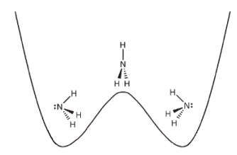
The two states of ammonia are stable equilibria of the potential energy, but the potential can be overcome and result in an atomic transition. Diagram courtesy of LibreTexts.
Such a system can occupy two states: the lower-energy state, which we will call (represented in the above diagram with the ammonia molecule on the left), and the higher-energy state, which we will call (represented by the ammonia molecule on the right). It is also common to refer to as the lower state and as the upper state, and we will adopt this naming convention for the rest of this chapter. The general state of the system, assuming that transitions are forbidden (and thus ), is given by:
where are eigenstates of the system’s Hamiltonian assuming no transitions (which we will call ):
Now, this is only the case if transitions are forbidden (which is a requirement of time independence) - but we know that transitions between the lower state and upper states do certainly exist. Therefore, we must add time-dependence to the system, which means must become functions of time :
Generally, however, these transitions happen randomly, resulting in spontaneous emission, which we don’t want for lasers. This means that somehow, we must keep more ammonia molecules in the upper state and less in the lower state, a population inversion, for stimulated emission to occur frequently enough that it becomes the dominant mode of light (electromagnetic radiation) production, which is a prerequisite for lasing.
Let us now examine how to formulate what we have described using the theoretical framework of quantum mechanics. We are primarily interested in stimulated emission, so we will not describe spontaneous emission in this section, although the calculations are actually rather similar. We will use the treatment originating with Griffiths (in Introduction to Quantum Mechanics) for this.
Consider an applied electromagnetic field , where and is the frequency of the field. This is a classic (idealized) solution to Maxwell’s equations of electromagnetism. The Hamiltonian must then include both the “standard” Hamiltonian as well as the contribution from the electromagnetic field , which has a dependence on time due to the EM field. Thus the complete Hamiltonian is given by:
The inclusion of the external EM field Hamiltonian is crucial. Recall how we previously saw that an applied EM field raises an atom’s electrons to an upper state, allowing stimulated emission to occur. The term in the Hamiltonian, also called a perturbation term, expresses this fact.
Now, let us assume we have already solved for the eigenstates of , and these are given by where is the lower state and are the upper states. The eigenstates are orthonormal and thus satisfy . The state of the system can be written in terms of these eigenstates as:
Where are time-dependent coefficients (also called transition amplitudes) whose squared norm is the probability of finding each eigenstate at time . For simplicity, let’s consider a system with only two states: the lower state , which has energy , and one upper state , which has energy . This may seem like a ridiculous simplification, given that atoms often have dozens of energy levels, but often, the electron transitions relevant to lasers happen only between two energy levels, so this is a reasonable assumption (indeed this is true for the famous ammonia laser[5]). Then, the state of the system would be given by:
Where once again, remember that are both functions of time. We now aim to solve for and , the transition amplitudes. To do so, we plug into the Schrödinger equation , where, remember, . The resulting expression is rather long:
Which we can slightly simplify (by expanding the brackets) to:
But recall that since are eigenstates of , they satisfy:
So, substituting in, we find that the terms actually cancel quite nicely:
Meaning that we are left with simply:
Where again and . Since the eigenstates are orthonormal and thus obey , if we multiply by on all sides, we would have:
Which reduces to:
We can do some rearranging (dividing by and multiplying by on both sides) to get on one side, leaving us with an ODE for :
Repeating the same process, only multiplying by rather than , gives us an ODE for :
The system of ODEs for and can be rewritten in matrix form (where here, as with before), just as we previously saw in the matrix representation section:
Let us assume that at time , the atom is in its upper state with energy . Thus the initial condition would be 100% probability of the state and 0% probability of the state:
We want to solve for , which will give us the probabilities of the atom decaying to the lower state at some future time (remember, even in stimulated emission, the decay time is random, only the probability of a decay is predictable). The differential equations are indeed quite intimidating to solve. There are, however, some steps we can use to simplify. First, the diagonals of the matrix are often zero; see this physical argument on Physics SE which explains why, which reduces each of the ODEs by one term, so that we “only” have:
We can then make use of a perturbative expansion. Let’s first assume that are small, meaning that transition between the states (including decays) happen relatively infrequently. If the transition rates are small enough, we can assume that . If this is the case, then . If we substitute this value of into the top ODE of the matrix system (the ODE for , we have:
With this simplification, the ODE becomes solvable - the solution is:
If we substitute our applied EM field Hamiltonian, which has , then the solution (once you perform the integral) is:
Taking the squared norm of yields the probability of the transition from the upper state to the lower state, which we will denote :
Note that we can also write this in terms of the energy density of an electromagnetic wave, , as:
We should add one more caveat: this is for a monochromatic applied electric field with a strict linear polarization. In practice, an applied electric field would be composed of many different frequencies, and would be a mix of different polarizations (for example, sunlight ranges from 300 to 2500 nm and is certainly unpolarized by the time it reaches Earth)[8]. In that case, instead of a single energy density, we instead have a spectral energy density , which gives the electromagnetic energy density at frequency . Recall again that Planck’s law of blackbody radiation tells us that this can be approximated by:
Where is the Boltzmann constant is the temperature, and . In this case, the more general expression for the probability of the transition via stimulated emission (which we will not derive) is:
Taking the time derivative of the transition probability gives us the transition rate, the probability of a transition per unit time. In fact, with the exception of a factor to make the units consistent (due to how the Einstein coefficients are defined), this is what we know to be the Einstein B coefficient:
And the Einstein coefficients in the rate equations are given by:
From which we may solve the rate equations that govern the population of the and states, which, as a reminder, are given by:
Note that the mean lifetime of the upper state, meaning the average amount of time an atom spends in the upper state before decaying into the lower state , can be calculated from the Einstein A coefficient as follows:
Of course, this is for just a two-level system (with one upper state and one lower state). Many lasers are three-level or four-level systems, and thus do not have such simple expressions for finding the transition probability. In the most complicated of cases, numerical methods can be used for solving the matrix ODEs to find the transition rates and the rate equations to solve for the population of each state.
Fermi’s golden rule
Our quantum model of lasers is actually just one example in the broader field of time-dependent perturbation theory, which describes the dynamics of multi-state quantum systems (like lasers!) Just as we saw at the very beginning of our discussion, time-dependent perturbation theory allows for the possibility of transitions between states. For such a system, we write out a Hamiltonian in the following form, just like we did for analyzing lasers:
Where is the time-independent Hamiltonian, and is the perturbation Hamiltonian, which is responsible for the time-dependent behavior of the system. Fermi’s golden rule says that to first-order, the probability of a transition per unit time from initial state to final state is given by:
Where is the density of states at energy , which we’ll explain in a little bit, and is called the matrix element for the transition, which is given by:
Fermi’s golden rule is applicable to a broad range of multi-state quantum systems, from nuclear physics to scattering processes described in quantum field theory (for those interested, becomes the first-order term of the S-matrix in QFT). The mean lifetime of the state before a decay to state can also be found from the transition rate via:
Using the transition rate, one may then find the following differential equation relating the population of state with the population of the state , which are simply the exponential decay/growth equations, assuming that there are no other transitions than the transition :
This looks very similar to the laser rate equations for a two-level system! Indeed, that is almost correct.
In our case of lasers, is , the Einstein A coefficient, and therefore is the lifetime of the upper state. Our entire process of finding and and calculating the transition probability could have been avoided, had we used Fermi’s golden rule directly. It is a very powerful tool to use when doing calculations.
The characteristics of laser light
At the very start of our discussion of lasers, we noted that lasers produce light with very specific characteristics:
Monochromatic light: The light is of one frequency (or essentially one frequency)
Directionality: The laser beam travels in one direction and can be focused tightly
Amplification: The emission of one photon triggers the emission of two more, starting a chain reaction that leads to a cascade of light, and making it possible to create powerful beams of light
With all we’ve learned, we can now answer the question of why laser light has these properties. First, the reason why light from a laser is only of one frequency comes directly from the stimulated emission process. Remember that since stimulated emission always produces two identical photons, which have identical frequencies. Since those two photons go on to trigger the emission of two more identical photons each (so four photons total), we have a chain reaction that continues, doubling the number of photons each time. This means that eventually, (nearly) all the photons in the optical cavity will be produced by stimulated emission, and they will be identical to each other, giving laser light its characteristic monochromaticity. However, this is only possible because lasers maintain a population inversion, since stimulated emission is only favored when the upper state has a higher population than the lower state. Normal light sources do not maintain a population inversion, so spontaneous emission dominates over stimulated emission, and as a result, their light is spread over a range of frequencies and is not monochromatic.
Second, the reason why laser light exhibits strong directionality is due to the mirrors in the laser’s optical cavity. We’ll first start by giving a more intuitive but less rigorous explanation. Imagine a photon that is emitted by stimulated emission, inside the optical cavity: if the photon’s direction is not exactly normal (90 degrees) to the mirror, it will reflect off the mirror at an angle, causing it to eventually hit the walls of the optical cavity, where it is absorbed and can no longer be reflected. Only photons normal to the mirror can get reflected again at the mirror on the other side, where they can continue travelling through the optical cavity.
The more complicated but also more rigorous explanation comes in the form of the wave nature of light. Light is an electromagnetic wave, and electromagnetic waves exhibit interference: when two waves are added together, if they have a different phase, they will interfere with each other. An electromagnetic wave that propagates along the optical axis (normal to the mirror) and another wave propagating at an angle to the optical axis would have a different phase, because two waves travelling over different distances will always have a phase difference proportional to the difference in the distances. Normally, we don’t notice this, because light travels so fast (it can travel around the Earth in 1/6th of a second!) that any phase shift is far beyond anywhere we could see. But in the closed optical cavity of a laser, surrounded by reflecting mirrors, small differences in phase add up as the electromagnetic waves reflect back-and-forth between the mirrors, quickly (in fact near-instantly) building up to the point that constructive interference leads to the waves along the optical axis to add up, and destructive interference leads to the waves that are at an angle to be cancelled out. This means we’re just left with waves travelling parallel to the optical axis, giving us a highly-directional, straight beam, whose power is concentrated along the direction of the beam.
Technically speaking, the emission of a photon from the state transition (decay from the upper state to a lower state) doesn’t happen completely on its own. The quantum electrodynamical vacuum is what mediates the transition and thereby the release of a photon, but that is an advanced topic we’ll cover in the expert guide